In this series of posts, I want to put some of my or my collaborators’ results in combinatorics of trees in a concrete form. I want to show how mathematical theorems sometimes can be translated almost verbatim into Haskell code. In the first part, I will discuss the counting results about coalescent histories.

For the necessary background to this post, please check out a small introduction into phylogenetic trees. In that post, I have defined species and gene trees as focal objects of modern phylogenetics. The essence of it is that a species tree describes the natural history of speciation events for a group of species, and a gene tree represents the relationship between genetic lineages sampled from these species. So, the two trees are closely related, but at the same time they can have different shapes (topologies).

A scientist would immediately pose an inference problem: “Can we learn about the species tree given a set of gene trees build from different chunks of DNA?”. That is a very valid question, and dozens of people are still working on in. A mathematician like me, however, wants to ask a different question: “Can we characterize the relationship between the two trees?”

In my opinion, that’s an amazing question because it’s very easy to formalize and prove theorems about. So, let me give you one way to think rigorously about this situation. What is the thing we care about in gene trees? It’s the coalescences, i.e. the nodes of the tree, since these are the events we can “observe” from our data (sample). They are discrete events that happen in the timespan of one generation. In short, in gene trees, we care about the nodes.

No one really observes real speciation events, except for some small-scale experiments. An event is usually declared a speciation only after the fact, when the two new species have sufficiently diverged from each other. So, in species trees, we care about the edges.

Now, our collective brain suddenly clicks: coalescences of the gene tree happen inside branches of the species tree. This looks like a function! This leads us to the main definition of the post.

Definition. Consider a pair of trees \((G,S)\) that are binary, rooted, and leaf-labeled, with the labels in bijective correspondence. Let \(G\) be the gene tree and \(S\) be the species tree. A coalescent history is a function \(\alpha\) from the set of internal nodes of \(G\) to the set of internal edges of \(S\), satisfying two conditions:

1. For each internal node \(v\) in \(G\), all labels for leaves descended from \(v\) in \(G\) label leaves descended from edge \(\alpha(V)\) in \(S\).

2. For each pair of internal nodes \(v_1\) and \(v_2\) in \(G\), if \(v_2\) is descended from \(v_1\), then \(\alpha(v_2)\) is descended from \(\alpha(v_1)\) in \(S\).

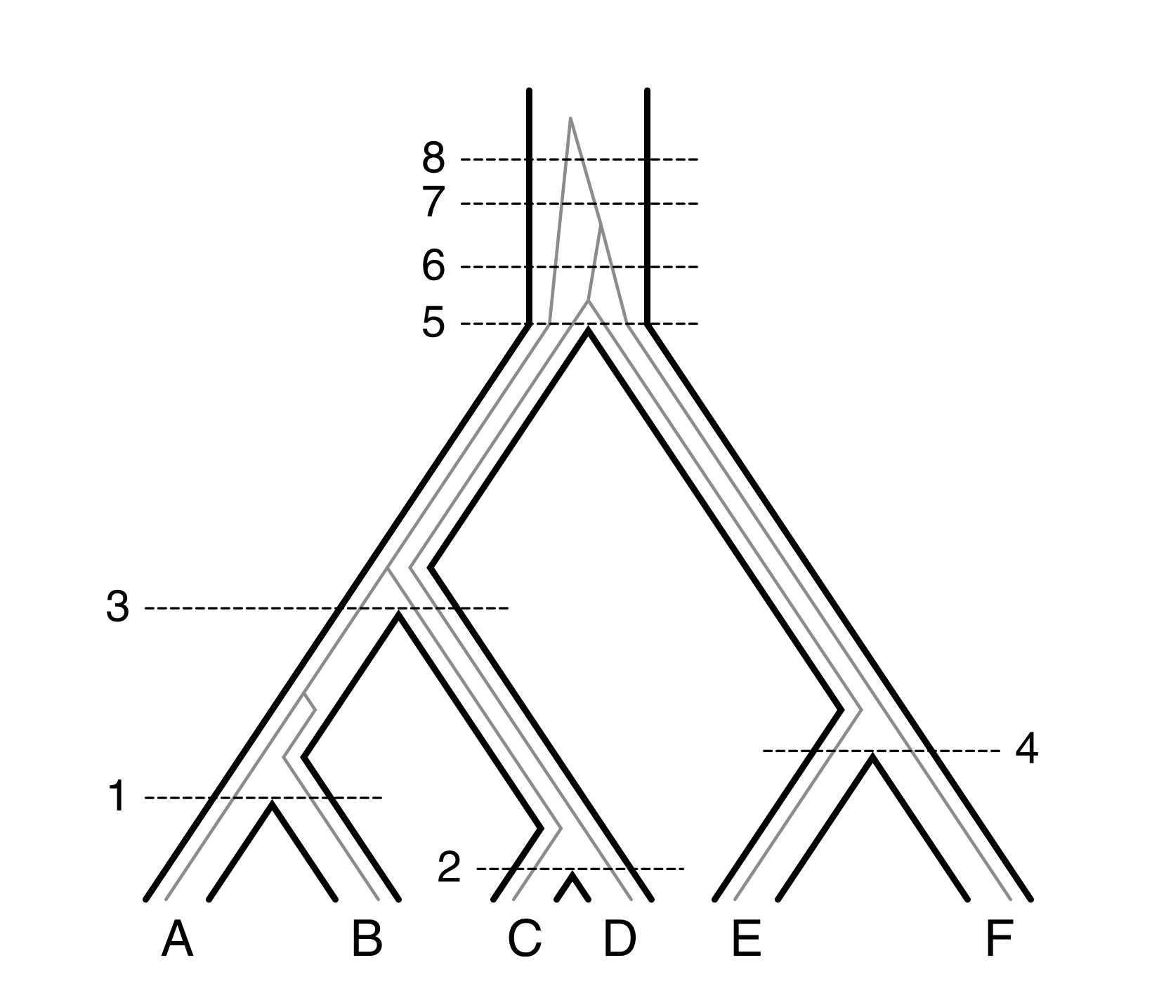
The conditions in this definition simply ensure that the tree “structure” is preserved: for example, ancestors cannot be mapped to an edge below their descendants. It is worth to take a minute to wrap your head around this definition. Here is a picture to help with it.

Matching case

How many coalescent histories are there? We are going to answer this counting question. Thankfully, all math has already been done for us by Professor Rosenberg. Let’s see what he says in his paper titled “Counting coalescent histories”.

Theorem. (Theorem 3.1, Rosenberg (2007)) For \(m \geq 1\) , the number of valid \(m\)-extended coalescent histories for a tree \(S\) with \(n \geq 2\) taxa is

\[A_{S,m} = \sum_{k=1}^m A_{S_L, k+1} A_{S_R,k+1},\]

where \(S_L\) and \(S_R\) respectively denote the left and right subtrees of \(S\). If \(S\) has \(n = 1\) taxon, then \(A_{S,m} = 1\) for all \(m\).

Okay, let’s figure it all out: what are \(m\)-extended coalescent histories? These are just the regular coalescent histories, but we subdivide the root of the species \(S\) artificially into \(m\) different edges. You can actually see this in Figure 1 above.

Okay, but why do we only have one tree here? This is actually the result for the case when the species tree and gene tree do have the same topology. I will cover the general result below.

Okay, okay, so the answer is just a recursive function? Yes, exactly! Trees are by their nature recursive structures, so it’s no surprise we got this answer. The base case is when the tree has a single leaf edge, no matter how many branches we have subdivided it into, and the big equation defines the recursive case.

Great, so what are the values of this function? Let’s find that out! We are finally ready to code this function.

The final result of this section is available in the companion repository: github.com/EgorLappo/tree_combinatorics_functions. It includes a small parser, allowing conversion between Haskell trees and string representations with parseString, and a rudimentary pretty-printing of trees in the form of a custom Show instance.

Let’s begin. Since I am using Haskell, I will start with defining our types. Here it is:

data Tree a = Leaf a | Node a (Tree a) (Tree a) deriving Eq

There are many helper functions that we may need in the future, and all of them are located in this file. I won’t reproduce all of them here, but here is an example function:

-- get all leaf labels
leafLabels :: Tree a -> [a]
leafLabels (Leaf a) = [a]
leafLabels (Node _ l r) = leafLabels l ++ leafLabels r

The theorem I am implementing is actually talking about extended trees that have a subdivided root edge. Here is the corresponding definition.

-- data type for m-extended trees
-- an extra `Int` records the subdivision of the branch
data ExtTree a = Leaf Int a | Node Int a (ExtTree a) (ExtTree a)

fromTree :: Tree a -> ExtTree a
fromTree (T.Leaf a) = Leaf 1 a -- kind of unnecessary in practice...
fromTree (T.Node a l r) = Node 1 a (fromTree l) (fromTree r)

toTree :: ExtTree a -> Tree a
toTree (Leaf _ a) = T.Leaf a
toTree (Node _ a l r) = T.Node a (toTree l) (toTree r)

labelExt :: ExtTree a -> a
labelExt (Leaf _ a) = a
labelExt (Node _ a _ _) = a

relabelExt :: Int -> ExtTree a -> ExtTree a
relabelExt k (Leaf _ a) = Leaf k a
relabelExt k (Node _ a l r) = Node k a l r

I have defined a new type of trees, ExtTree, that keep information about branch subdivisions as an integer. There is also a pair of natural transformations between the regular Trees and ExtTrees, as well as very important helper functions that work with numberings and labels of the tree root.

With this small bit of preparation, the theorem takes just a few lines:

-- helper to match the type
countMatchingCoalescentHistories :: Tree a -> Int
countMatchingCoalescentHistories = 
  countMatchingCoalescentHistories' . fromTree

-- Rosenberg (2007), Thm 3.1
countMatchingCoalescentHistories' :: ExtTree a -> Int
countMatchingCoalescentHistories' (Leaf _ _) = 1
countMatchingCoalescentHistories' (Node m _ l r) = (sum . zipWith (*)) aL aR
  where sLs = [relabelExt (k+1) l | k <- [1..m]]
        sRs = [relabelExt (k+1) r | k <- [1..m]]
        aL = map countMatchingCoalescentHistories' sLs
        aR = map countMatchingCoalescentHistories' sRs

If you know Haskell syntax, this function should be barely different from the plain-text statement of the theorem. If the tree is a Leaf (with any label and subdivision), the result is just \(1\). If we have a node instead, we compute the recursive cases and combine them. The sum . zipWith (*) function is responsible for the aggregation of the values computed on subtrees. The values recursively computes values are aR and aL. They are computed by applying our function to left and right subtrees that have been extended by k+1, just as in the statement of the theorem. Note that by using fromTree, we make sure that we count \(1\)-extended coalescent histories when we call countMatchingCoalescentHistories, which is exactly what we were after.

Ok, great! This was simple and easy. Let’s use it to generate some numbers!

ghci> let trees = map parseString ["(a,b)", "((a,b),c)", "(((a,b),c),d)", "((((a,b),c),d),e)"]

ghci> map countMatchingCoalescentHistories trees
[1,2,5,14]

The numbers 1, 2, 5, 14 are the very famous Catalan numbers! They appear naturally as the number of coalescent histories for “catepillar” trees.

Nonmatching case

Now let’s do the harder case in which the shape of the gene tree is different from the species tree. We have to consult the paper by Dr. Rosenberg once again.

Definition (Def. 4.1, Rosenberg (2007)). For a tree \(S\) with \(n \geq 2\) taxa and a tree \(G\) whose taxa are a subset of those of \(S\), let \(T(G,S)\) denote the minimal displayed tree of \(S\) that is induced by the taxa of \(G\).

Definition (Def. 4.2, Rosenberg (2007)). For a tree \(S\) with \(n \geq 2\) taxa and a tree \(G\) whose taxa are a subset of those of \(S\), let \(d(G,S)\) denote the number of branches of \(S\) that separate the root of \(S\) from the root of \(T(G,S)\). For a given tree \(S\), considering all possible trees \(G\) whose taxa form a subset of those of \(S\), the value of \(d(G,S)\) ranges from \(0\) to the largest number of branches separating a leaf from the root of \(S\).

Theorem (Thm. 4.3, Rosenberg (2007)) For \(m \geq 1\), the number of valid \(m\)-extended coalescent histories for a species tree labeled topology \(S\) with \(n \geq 2\) taxa and a gene tree labeled topology \(G\) whose taxa are a subset of those of \(S\) is

\[ B_{G,S,m} = \sum_{k=1}^m B_{G_L, T(G_L,S),k+d(G_L,S)} B_{G_R, T(G_R,S),k+d(G_R,S)}\]

where \(G_L\) and \(G_R\) respectively denote the left and right subtrees of \(G\). If \(n = 1\) or \(G\) has only one taxon, then \(B_{G,S,m} = 1\) for all \(m\).

Wow, this no longer looks like a simple recursion! Let’s first understand all the new terms. The function \(T(G,S)\) intuitively corresponds to the following operation: find all the leaves in \(G\) among the leaf labels of \(S\), and then return the tree “below” the most recent common ancestor of these leaves in \(S\). The point here is that \(T(G,S)\) may contain other leaves that are not part of \(G\). For example, take \(G=(a,c)\) and \(S=((a,b),c)\). Then, \(T(G,S) = S\) (think through this!).

The function \(d(G,S)\) is pretty self explanatory. It determines how many extra subdivisions of branches we need to introduce to account for nonmatching topologies.

It turns out that, despite having two different trees here, we are still recursing on the gene tree \(G\). The species tree plays an auxiliary function, letting us compute \(T(G,S)\) and \(d(G,S)\). So, it must be possible to elegantly express this with Haskell.

countNonmatchingCoalescentHistories :: Eq a => Tree a -> Tree a-> Int
countNonmatchingCoalescentHistories g s 
  = countNonmatchingCoalescentHistories' (fromTree g) (fromTree s)

countNonmatchingCoalescentHistories' :: Eq a => ExtTree a -> ExtTree a -> Int
countNonmatchingCoalescentHistories' (Leaf _ _) _ = 1
countNonmatchingCoalescentHistories' _ (Leaf _ _) = 1
countNonmatchingCoalescentHistories' (Node _ _ gl gr) s@(Node m _ _ _) 
  = sum $ zipWith (*) bL bR
    where 
       tl = (fromTree . mrcaNode (toTree s) . leafLabels . toTree) gl
       tr = (fromTree . mrcaNode (toTree s) . leafLabels . toTree) gr
       dl = length $ ancestorNodes (labelExt tl) (toTree s)
       dr = length $ ancestorNodes (labelExt tr) (toTree s)
       bL = [countNonmatchingCoalescentHistories' gl (relabelExt (k + dl) tl) | k <- [1..m]]
       bR = [countNonmatchingCoalescentHistories' gr (relabelExt (k + dr) tr) | k <- [1..m]]

This is quite a bit more involved than the matching case, but we can still get through it! The first thing to notice is that now we have two “terminating” cases for the recursion: one for \(G\) and one for \(S\).

The second thing is that the structure of the function is the same: there is the “aggregation pattern” sum . zipWith (*) and recursively computed values in lists bL and bR.

To compute \(T(G,S)\), I compose two functions:

t g s = mrcaNode s (leafLabels g)

First, get the leaf labels of g, and then find their most recent common ancestor in s – done! I just need to wrap this with tree transformations to make the helper functions work with the extended tree type. To compute \(d(G,S)\) I compute the length of the chain of ancestors from the root node of \(T(G,S)\) to the root of \(S\), also using a helper function.

The function leafLabels, mrcaNode, and others can be found in this file.

You can try downloading my repository and running the code yourself! Try to find some more interesting number sequences using the nonmatching function. I hope this little tutorial was useful!