Check out Part I of this series first!

For the necessary background to this post, please read a small introduction into phylogenetic trees. In that post, I have defined species and gene trees as focal objects of modern phylogenetics. The essence of it is that a species tree describes the natural history of speciation events for a group of species, and a gene tree represents the relationship between genetic lineages sampled from these species. So, the two trees are closely related, but at the same time they can have different shapes (topologies).

In this post, I will offer another mathematical perspective on the relationship between gene and species trees: ancestral configuration. We will once again consult the papers for definitions and theorems, and then implement this structure with Haskell.

Coalescent histories were essentially maps from nodes of the gene tree into the branches of the species tree that satisfy some natural conditions. Ancestral configurations are not maps but sets of lineages, i.e. sets of edges of the gene tree.

To define ancestral configurations, we need to talk about realizations. Given a gene tree \(G\) and a species tree \(S\), a realization \(R\) of \(G\) in \(S\) is essentially a juxtaposition of the “thin” tree \(G\) with the “thick” tree \(S\), just like in the illustration of the multispecies coalescent from the introductory blogpost. Here is how it looks:

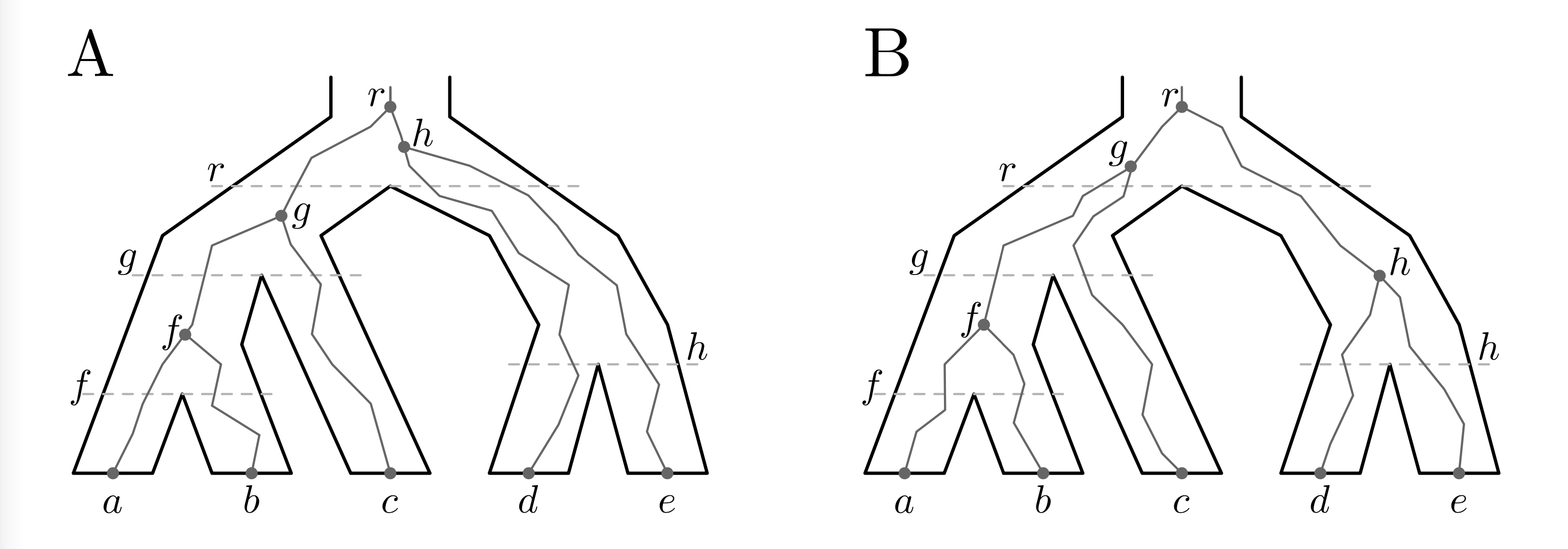
In these pictures we are interested in what happens at each node of the species tree. The horizontal lines representing nodes of \(S\) intersect some number of lineages (edges) of \(G\). The set of lineages of \(G\) intersecting a given node \(v\) of \(S\) is called an ancestral configuration at \(v\).

The set of ancestral configurations at \(v\) is denoted \(C(G,S,v)\). We are particularly interested in root ancestral configurations \(C(G,S,r)\). Let’s further restrict ourselves to the case \(G=S\) and let \(C(S) = C(S,S,r)\) be the set of root ancestral configurations of \(S\). For example, looking at Figure 1, we can see that in (A) the root ancestral configuration is \(\{g,d,e\} \in C(S)\), and in \(B\) it is \(\{f,c,h\} \in C(S)\). (Here I have labeled each lineage/edge using the same label as a node right below that edge.) For an extended definition, you can take a look at this paper.

What can we say about the set \(C(S)\)? Disanto & Rosenberg (2017) have an answer for us!

Given a tree \(S\), let \(\ell\) and \(r\) be the left and right root lineages (lineages adjacent to the root of \(S\). Also, let \(S|_\ell\) be the left root subtree, and \(S|_r\) be the right root subtree. Then, the authors prove the following result about \(C(S)\):

\[ C(S) = \{\{\ell,r\}\}\bigcup \left[C(S|_\ell) \otimes \{\{r\}\}\right] \bigcup \left[\{\{\ell\}\} \otimes C(S|_r)\right] \bigcup \left[C(S|_\ell)\otimes C(S|_r)\right], \]

where \(A\otimes B = \{a\cup b \mid a \in A, b\in B\}\) for sets of sets \(A\) and \(B\). Dealing with sets of sets is never simple, so the notation sucks. It’s okay though, we still will turn this into beautiful code.

The coding part

Ok, so we have our definitions and a result that we want to implement. We also already have a type for trees from part I:

data Tree a = Leaf a | Node a (Tree a) (Tree a) deriving Eq

Given some Tree a, we will represent the set of ancestral configurations as [[a]], which roughly corresponds to sets of sets above. With this, implementing the equation above is very simple.

rootConfigurations :: Eq a => Tree a -> [[a]]
rootConfigurations (Leaf _) = []
rootConfigurations (Node _ l r) = 
    [[label l, label r]]
 ++ [label l : rs | rs <- rootConfigurations r]
 ++ [ls ++ [label r] | ls <- rootConfigurations l]
 ++ [ls ++ rs | ls <- rootConfigurations l, rs <- rootConfigurations r]

label :: Tree a -> a
label (Leaf a) = a
label (Node a _ _) = a

We see the same four components, same structure, just with list concatenation instead of set union.

I will leave you with some homework today: write a function

nonmatchingRootConfigurations :: Eq a => Tree a -> Tree a -> [[a]]

for a nonmatching pair! Hint: try to generate matching configurations for the gene tree \(G\), and omit those that do not “fit” with \(S\). For a solution see this file and a reference to my paper in the comment.